Decision Trees and Ensemble Methods

Introduction

Decision trees occupy a somewhat special place in data science. They are among the first machine learning models that can be explained without heavy mathematics, yet they scale to surprisingly complex problems. At the same time, they expose some of the fundamental difficulties of learning from data.

In this chapter, we will first develop decision trees as a learning model from the ground up. Only once their strengths and weaknesses are clearly understood do we turn to ensemble methods, which can be seen as a systematic way of fixing precisely those weaknesses.

Throughout the chapter, we will repeatedly return to a small, concrete example, the Play Tennis dataset, to anchor abstract concepts in something tangible.

The goal is not to memorise algorithms, but to understand why they are constructed the way they are.

---

What is a decision tree?

At its core, a decision tree is a structured sequence of questions. Each question splits the input space into simpler regions until a final decision can be made.

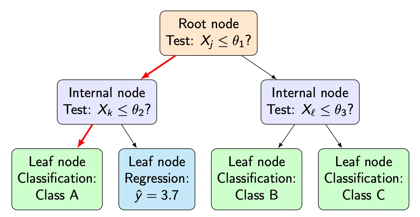
A few terms are essential:

• The root node is the starting point of the tree and represents the full dataset.
• Internal nodes contain decision rules, such as “Is humidity ≤ 75%?”
• Edges correspond to the outcome of a decision.
• Leaf nodes contain the final prediction.

For classification tasks, a leaf typically stores either a class label or a distribution over classes. For regression tasks, it usually stores a numerical value such as a mean.

At this stage, a decision tree is simply a data structure. Nothing has been learned yet.

---

Prediction as a deterministic process

To understand decision trees, it helps to first ignore learning entirely and focus on prediction.

Given an input vector $x$, prediction proceeds as follows:

1. Start at the root node.
2. Evaluate the decision rule stored at the node.
3. Follow the corresponding edge.
4. Repeat until a leaf node is reached.
5. Output the prediction stored in the leaf.

This process is fully deterministic. For a fixed tree and a fixed input, the same prediction will always be produced.

This property is one reason decision trees are often considered interpretable: the sequence of decisions can be inspected and explained step by step, both for the model designer and for the user.

---

Intuition before algorithms

Suppose we are given a small dataset about whether people decide to play tennis, depending on weather conditions such as outlook, humidity, wind, and temperature.

The dataset we will use throughout the chapter is shown below.

The Play Tennis dataset

Outlook	Temperature	Humidity	Wind	Play Tennis
Sunny	Hot	High	Weak	No
Sunny	Hot	High	Strong	No
Overcast	Hot	High	Weak	Yes
Rain	Mild	High	Weak	Yes
Rain	Cool	Normal	Weak	Yes
Rain	Cool	Normal	Strong	No
Overcast	Cool	Normal	Strong	Yes
Sunny	Mild	High	Weak	No
Sunny	Cool	Normal	Weak	Yes
Rain	Mild	Normal	Weak	Yes
Sunny	Mild	Normal	Strong	Yes
Overcast	Mild	High	Strong	Yes
Overcast	Hot	Normal	Weak	Yes
Rain	Mild	High	Strong	No

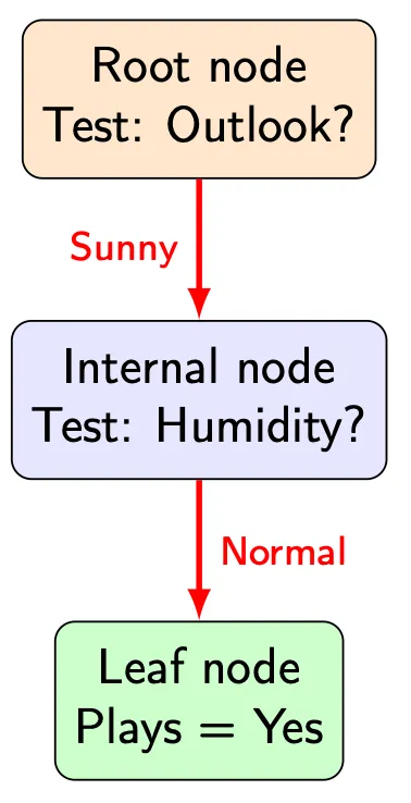
Before applying any algorithm, a human might immediately propose a simple tree.

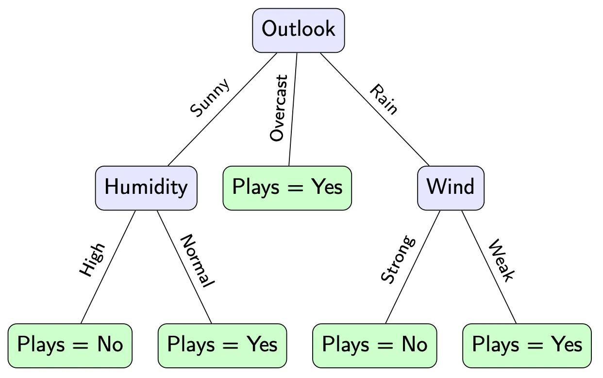
This kind of tree feels reasonable. It mirrors how people often reason: start with a prominent feature, then refine the decision if necessary.

However, this intuition hides an important question:

Why should this particular question come first?

So far, the structure of the tree is based on subjective judgment. If another person designed the tree, it might look quite different.

Learning a decision tree means replacing this intuition with a systematic criterion.

---

What does it mean to learn a tree?

Learning a decision tree means answering the following question repeatedly:

Which question should we ask next?

At each node, we must choose:

• a feature,
• and possibly a threshold or partition of its values,

such that the resulting child nodes are in some sense better than the parent node.

In the tennis example, this means deciding whether the first split should be based on Outlook, Humidity, Wind, or Temperature.

To make this decision systematic, we need a way to measure how “mixed” or “uncertain” a node is.

---

Measuring impurity

Consider again the root node of the Play Tennis dataset. It contains all 14 observations with the following class distribution:

Class	Count	Proportion
Yes	9	9 / 14
No	5	5 / 14

Intuitively, this node is not pure: both outcomes occur. To quantify how mixed the node is, we compute the Gini impurity.

Let

• $p_{\text{yes}} = \frac{9}{14}$
• $p_{\text{no}} = \frac{5}{14}$

The Gini impurity is defined as

$$G = 1 - \sum_k p_k^2$$

Plugging in the numbers gives

$$\begin{aligned} G &= 1 - \left(\frac{9}{14}\right)^2 - \left(\frac{5}{14}\right)^2 \\ &= 1 - \frac{81}{196} - \frac{25}{196} \\ &= 1 - \frac{106}{196} \\ &= \frac{90}{196} \approx 0.46 \end{aligned}$$

This value is neither close to 0 (perfectly pure) nor close to its maximum (highly mixed). It reflects exactly what we see in the data: most days lead to Yes, but a substantial number do not.

---

Why Gini impurity works

The Gini impurity can be understood through a simple probabilistic argument.

Consider a binary indicator variable $Y_k$ that takes the value

$$Y_k = \begin{cases} 1 & \text{if a sample belongs to class } k \\ 0 & \text{otherwise} \end{cases}$$

with probability $p_k$.

The variance of this variable is

$$\mathrm{Var}(Y_k) = p_k(1 - p_k).$$

Summing this variance over all classes yields

$$\sum_k p_k(1 - p_k) = 1 - \sum_k p_k^2,$$

which is exactly the Gini impurity.

From this perspective, Gini impurity measures how much class-related variability remains in a node, such as the mixed outcomes at the root of the Play Tennis dataset.

---

CART: Classification and Regression Trees

So far, we have discussed decision trees in a general sense. To make the learning procedure precise, we now focus on a specific and widely used framework: CART, short for Classification and Regression Trees.

CART is not a single algorithmic trick, but a well-defined family of decision tree methods introduced by Breiman et al in their seminal 1984 monograph. It specifies how trees are structured, how splits are evaluated, and how predictions are made.

In this chapter, when we talk about “decision trees”, we implicitly mean CART-style trees.

CART is characterised by three key design choices:

1. Binary splits only: Every internal node splits the data into exactly two child nodes. This is true even for categorical features with more than two possible values.

2. Greedy, top-down learning: The tree is built recursively. At each node, the split that looks best locally is chosen, without reconsidering earlier decisions.

3. Impurity-based split selection: For classification tasks, splits are chosen by maximising an impurity reduction (most commonly based on Gini impurity).

These choices strongly influence both the strengths and weaknesses of decision trees. In particular, the greedy nature of CART is one of the main reasons why decision trees tend to be high-variance models.

---

Choosing a split

With CART, learning a decision tree means repeatedly solving the following problem:

Given the samples at the current node, which binary split should be applied next?

At this point, we already know how to measure impurity at a node. What remains is to decide how impurity should be reduced.

Because CART allows only binary splits, categorical features must be partitioned into two disjoint subsets of values.

In the Play Tennis dataset, the feature Outlook takes the three values Sunny, Overcast, and Rain. Possible binary splits therefore include, for example:

• {Overcast} vs {Sunny, Rain}
• {Sunny} vs {Overcast, Rain}
• {Rain} vs {Sunny, Overcast}

Each of these splits leads to a different partition of the data. To choose between them, we need a precise numerical criterion.

Impurity reduction as the CART learning criterion

Let ( S ) denote the set of samples at the current node. A candidate split divides ( S ) into two subsets ( $S_\text{left}$ ) and ( $S_\text{right}$ )

The impurity after the split is defined as the weighted average

$$G_{\text{after}} = \frac{|S_\text{left}|}{|S|} \, G(S_\text{left}) + \frac{|S_\text{right}|}{|S|} \, G(S_\text{right})$$

What matters is the difference between the impurity before and after the split.

The impurity reduction is therefore defined as

$$\Delta G = G(S) - G_{\text{after}}$$

In CART, this quantity is the core learning signal. Among all candidate splits at a node, the split with the largest impurity reduction is selected.

Tree learning in CART consists of repeating this comparison recursively until a stopping criterion is reached.

Numerical example: splitting on Outlook

Consider the binary split

{Overcast} vs {Sunny, Rain}

The resulting class distributions are:

Group	Yes	No	Total
Overcast	4	0	4
Sunny ∪ Rain	5	5	10

---

Step 1: Gini impurity of each side

Overcast

All samples belong to class Yes:

$$G_{\text{overcast}} = 0$$

Sunny ∪ Rain

$p_{\text{yes}} = 5/10,\; p_{\text{no}} = 5/10$

$$G_{\text{sunny,rain}} = 1 - \left(\frac{5}{10}\right)^2 - \left(\frac{5}{10}\right)^2 = 0.5$$

---

Step 2: Impurity after the split

The weighted impurity is

$$\begin{aligned} G_{\text{after}} &= \frac{4}{14} \cdot 0 + \frac{10}{14} \cdot 0.5 \\ &= \frac{5}{14} \approx 0.36 \end{aligned}$$

---

Step 3: Impurity reduction

The impurity at the root node was

$$G_{\text{before}} \approx 0.46$$

The impurity reduction is therefore

$$\Delta G = 0.46 - 0.36 \approx 0.10$$

This value quantifies how much uncertainty is removed by asking “Is the outlook Overcast?”

---

Comparing all candidate splits at the root

For the root node of the Play Tennis dataset, CART evaluates all possible binary splits of each feature. The resulting impurity reductions are shown below.

Feature	Test (value)	Impurity Reduction ΔG
Outlook	∈ {Overcast}?	0.1020
Outlook	∈ {Sunny}?	0.0655
Outlook	∈ {Rain}?	0.0020
Temperature	∈ {Hot}?	0.0163
Temperature	∈ {Cool}?	0.0092
Temperature	∈ {Mild}?	0.0009
Humidity	∈ {High}?	0.0918
Humidity	∈ {Normal}?	0.0918
Wind	∈ {Weak}?	0.0306
Wind	∈ {Strong}?	0.0306

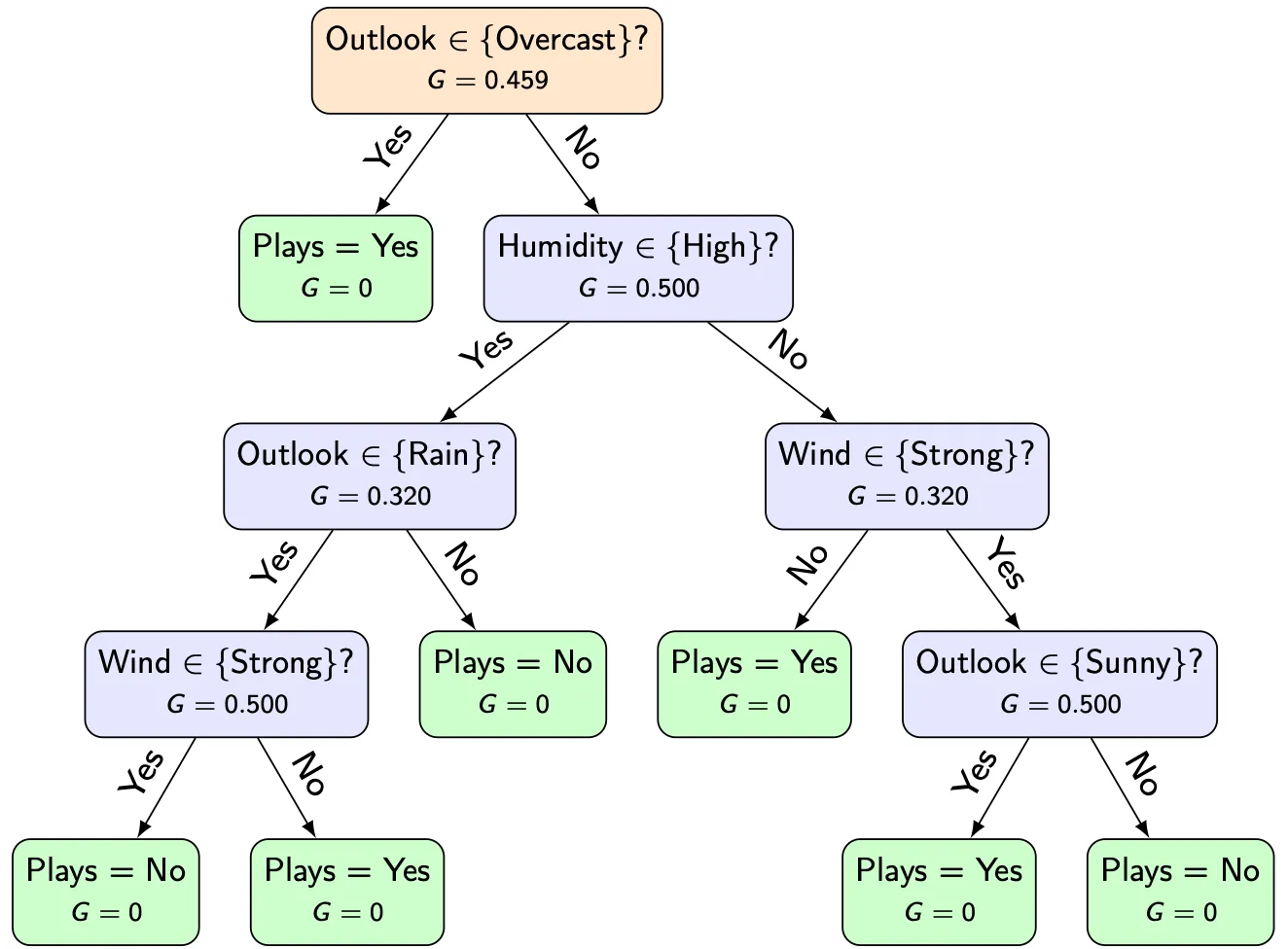
The split that isolates Overcast yields the largest impurity reduction. This is why it becomes the first decision in the learned tree.

---

Building the tree recursively

Once the best split at the root node has been chosen, the same procedure is applied recursively to each child node.

For example, after splitting by Outlook, the algorithm considers only the samples in the Sunny branch and asks again which feature should be used next.

This greedy strategy continues until a stopping condition is reached.

The result is a fully specified decision tree.

---

The central weakness of decision trees

Decision trees are flexible and easy to interpret, but they suffer from a fundamental problem: high variance.

Small changes in the training data, such as removing or duplicating a single tennis day, can lead to noticeably different trees. This instability is not a flaw of a particular implementation, it is inherent to the greedy nature of tree learning.

The natural question is therefore:

Can we keep the expressive power of trees while reducing their instability?

---

From single models to ensembles

A simple idea from statistics provides a hint: averaging reduces variance.

If we train many different decision trees on slightly different versions of the Play Tennis dataset and average their predictions, the result is often more stable than any individual tree.

This idea forms the basis of ensemble methods.

---

Bagging: bootstrap aggregating

Bagging combines decision trees with resampling.

The procedure is as follows:

1. Draw multiple bootstrap samples from the training set.
2. Train one decision tree on each bootstrap sample.
3. Aggregate the predictions:
   • majority vote for classification,
   • mean for regression.

Each individual tree may overfit peculiarities of its own bootstrap sample. Averaging across many such trees reduces this effect.

---

Why bootstrap sampling matters

Sampling with replacement ensures that:

• some tennis days appear multiple times in a training set,
• others are omitted entirely.

This introduces variation between the trees even though the same learning algorithm is used.

Without this variation, averaging would not meaningfully reduce variance.

---

Random forests: reducing correlation further

Random forests extend bagging by adding a second source of randomness.

In addition to bootstrap sampling, each split considers only a random subset of features.

In the Play Tennis example, this means that a tree might be forced to choose between Humidity and Wind at a node, even if Outlook would otherwise dominate.

This reduces correlation between trees and makes averaging more effective.

---

A brief note on boosting

Bagging and random forests rely on averaging many independent models.

Boosting follows a different philosophy: models are trained sequentially, each focusing on correcting the errors of the previous ones.

Boosting methods can be extremely powerful, but they also require more careful tuning.

---

Summary

Decision trees provide a clear and intuitive model for supervised learning, but they are inherently unstable.

By revisiting the tennis example throughout this chapter, we have seen how:

• trees are built by greedily reducing impurity,
• small data changes can strongly affect their structure.

Ensemble methods transform this weakness into a strength:

• bagging stabilises trees through averaging,
• random forests further reduce correlation through feature randomness.

Seen this way, ensembles are not an add-on, but a natural continuation of the decision tree idea.

---

Slides