Creating Heave-Corrected Echograms with echopype

Motivation

When working with vertically oriented echosounder data, creating an echogram often looks deceptively simple: “compute Sv, plot it against time and depth, done.” In practice, however, small details in the processing pipeline can have a surprisingly large impact on how the final echogram looks and whether it is physically interpretable at all.

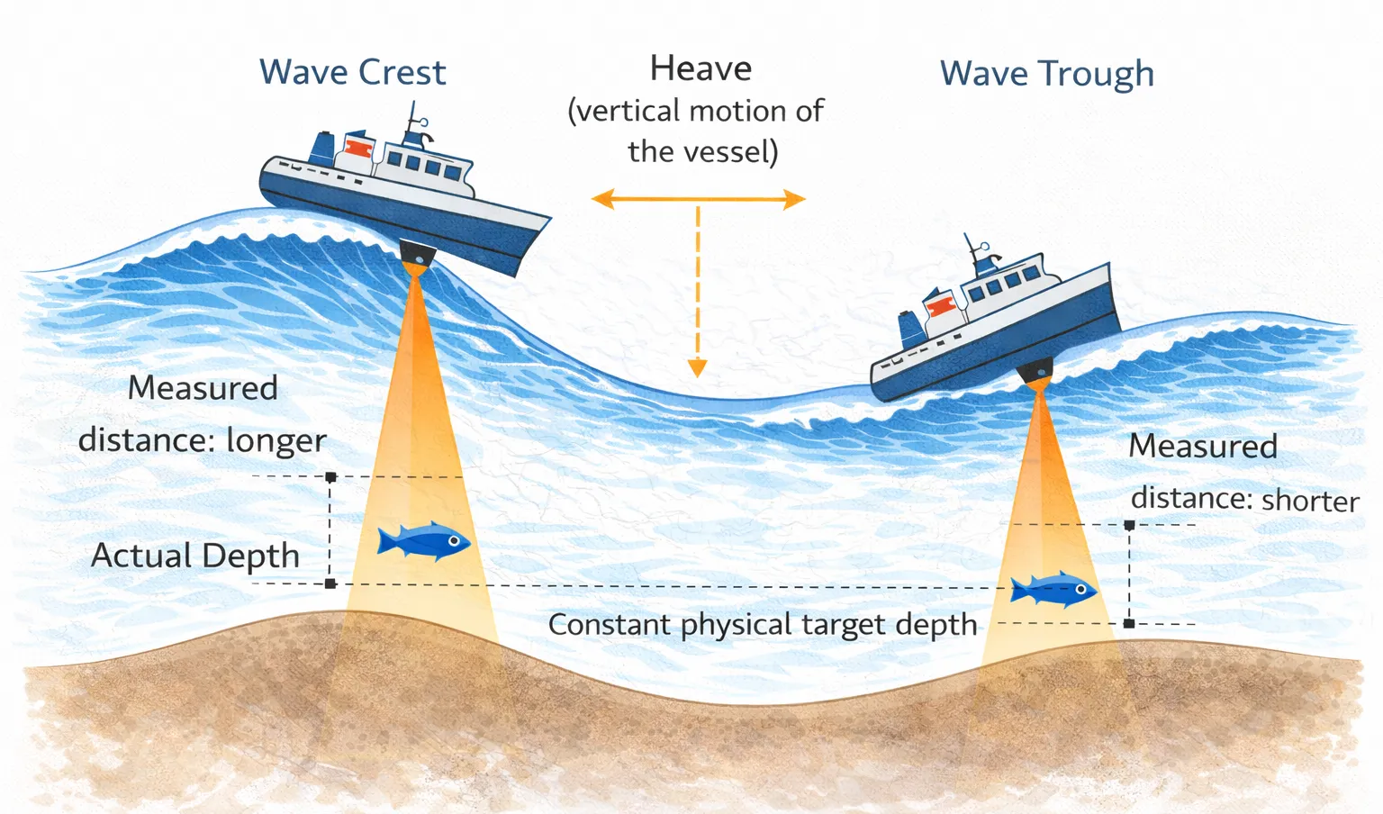
One such detail is vessel heave.

It took me longer than I would like to admit to understand where heave information is stored in echopype and how it actually affects the depth coordinate. I would have benefited from a short, explicit example that ties these pieces together. This post is an attempt to write exactly that.

Context of the example

The workflow shown below is not meant as a universal template, but as a concrete, reproducible example. The results and figures in this post are based on the following setup:

• echopype version: >= 0.11.0 (this is the only strict requirement — earlier versions handle depth consolidation differently)
• Data state: the data have already been converted using echopype and are opened via open_converted (for raw EK80 files, the equivalent entry point would be open_raw)
• Instrument and geometry: EK80 echosounder, oriented vertically downward
• Temporal subset: one short “Haul” segment, roughly 30 minutes long
• Storage format: Zarr (.zarr) for convenience and fast iteration

None of these choices are strictly required to apply heave correction in echopype. They simply define the concrete scenario on which the examples and figures in this post are based.

Opening the converted dataset

We start by opening the converted Zarr dataset. At this stage, no calibration or consolidation has been applied yet.

import echopype as ep

ed = ep.open_converted("./example_data/haul.zarr")

The resulting EchoData object contains both the acoustic measurements and the platform-related information needed later for depth calculation.

Where heave enters the picture

A key realization - and the main motivation for this post - is the following:

Heave information is stored in:

ed.platform["vertical_offset"]

This variable represents the vertical displacement of the transducer over time due to vessel motion.

In the context of a vertically downward-looking echosounder, this matters because all ranges are initially measured relative to the transducer. If the transducer moves up and down, the same physical target will appear at different apparent depths unless this motion is accounted for explicitly.

Before doing anything else, it is worth checking whether vertical_offset actually varies over time:

ed.platform["vertical_offset"].plot()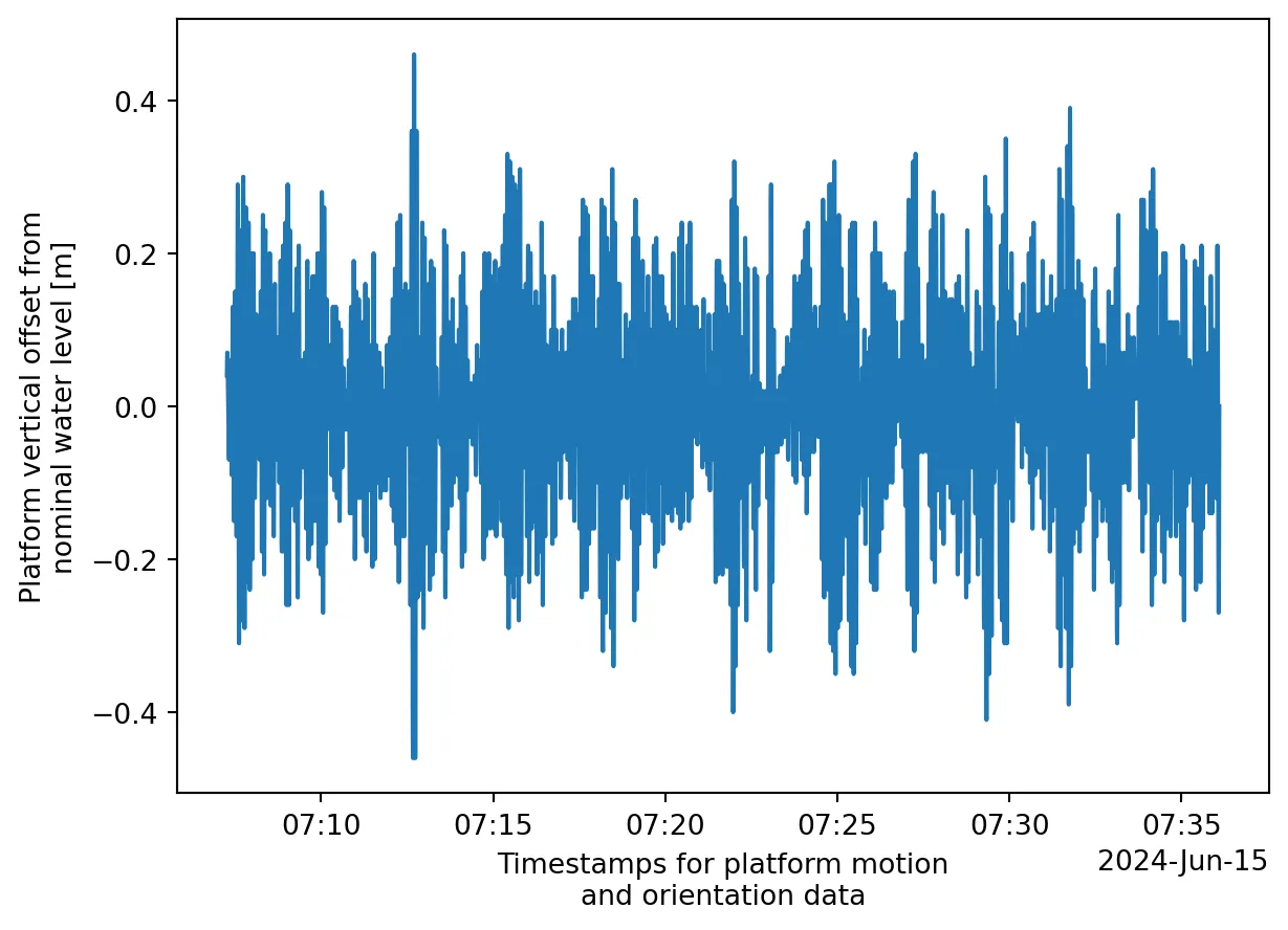

If this time series is constant, heave correction will have little effect. If it varies, ignoring it will introduce artificial vertical structure into the echogram.

Computing Sv and adding depth

We now compute the volume backscattering strength and convert range to depth.

ds_Sv = ep.calibrate.compute_Sv(
    ed,
    waveform_mode="CW",
    encode_mode="power"
)

At this point, the data are still range-based. To obtain a physically meaningful depth coordinate, we use add_depth:

ds_Sv = ep.consolidate.add_depth(
    ds_Sv,
    ed,
    use_platform_angles=True,
    use_platform_vertical_offsets=True
)

The crucial parameter here is use_platform_vertical_offsets=True. This is what incorporates heave into the depth calculation.

After this step, depth is no longer a simple one-dimensional coordinate. Instead, it becomes a two-dimensional coordinate that varies with both ping_time and range_sample.

This detail is easy to overlook, but it fundamentally changes how the data should be interpreted.

Basic data sanity checks

Before plotting, it is worth performing a small number of defensive checks.

First, we ensure that time is strictly increasing:

eqc.exist_reversed_time(ds_Sv, "ping_time")

Reversed timestamps are rare, but if present, they can silently break downstream processing.

Cleaning the depth coordinate

In practice, the computed depth coordinate may contain missing values, for example during brief motion irregularities. While this does not necessarily invalidate the data, it complicates plotting and aggregation.

A pragmatic solution is to interpolate missing values in both dimensions:

depth2d = ds_Sv["depth"]

depth2d_clean = (
    depth2d
    .interpolate_na(dim="ping_time", method="linear")
    .interpolate_na(dim="range_sample", method="linear")
    .ffill("ping_time").bfill("ping_time")
    .ffill("range_sample").bfill("range_sample")
)

ds_Sv = ds_Sv.assign_coords(depth=depth2d_clean)

This does not add new information, but it stabilizes the depth grid and makes subsequent visualization more robust.

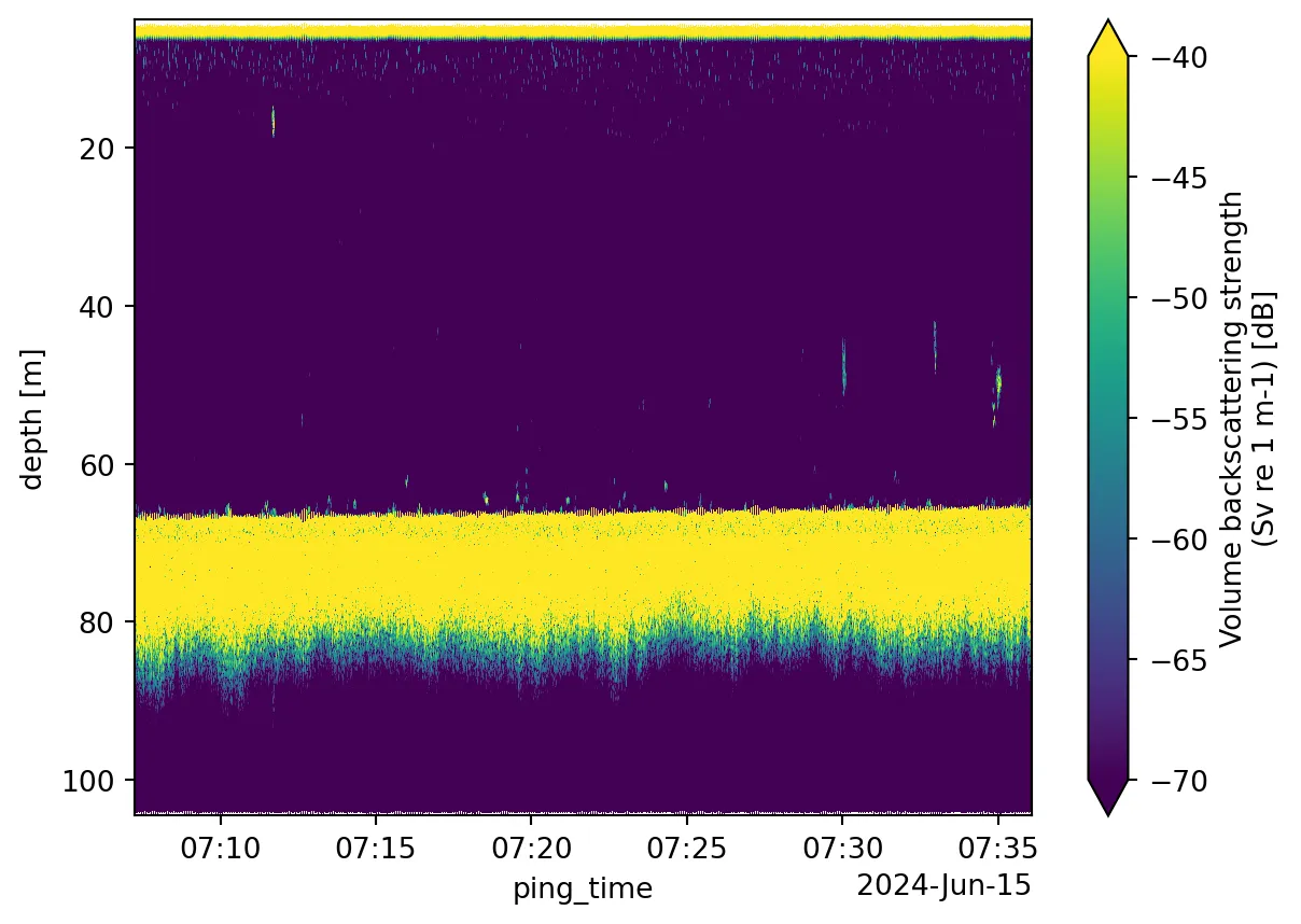
Plotting the echogram

We now select a single channel and plot the echogram. In fisheries acoustics, the 38 kHz channel is commonly used as a proxy for bulk biomass and is less sensitive to small scatterers.

# Take the one you find most appropriate
channel = 3
ch = ds_Sv["channel"].values[channel]

ds_Sv["Sv"].sel(channel=ch, drop=True).plot(
    x="ping_time",
    y="depth",
    yincrease=False,
    vmin=-70,
    vmax=-40,
)

Two small but important details:

• yincrease=False ensures that depth increases downward, matching physical intuition
• Fixing vmin and vmax makes different plots comparable and avoids misleading contrast

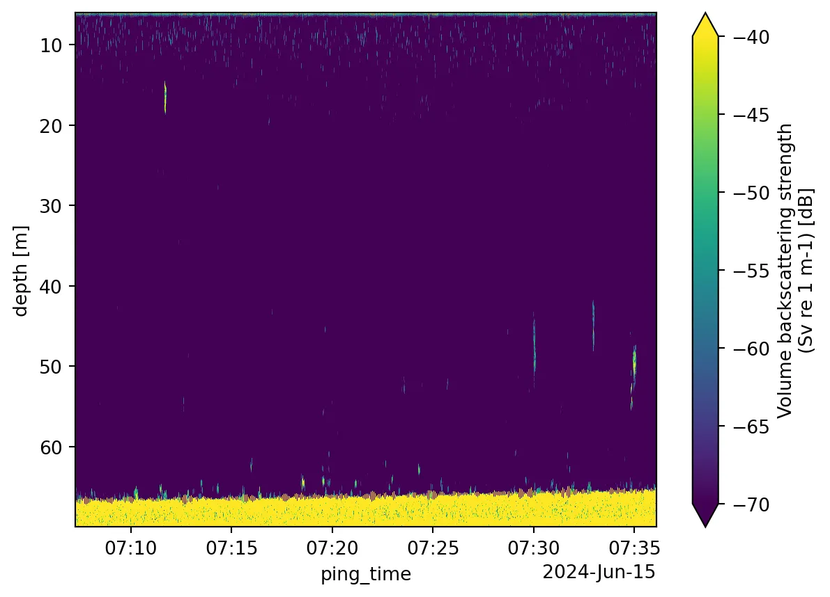
Constraining the depth range

In many cases, it is useful to restrict the depth range before interpretation.

Near-surface data are often dominated by vessel noise, bubbles, or flow effects. At the other extreme, everything below the seabed is artefactual by definition.

A simple mask can be applied as follows:

depth2d = ds_Sv["depth"]

mask = (depth2d >= 6) & (depth2d <= 70)
ds_Sv = ds_Sv.where(mask)

Upper and lower bounds are typically chosen based on a combination of vessel characteristics, known transducer depth, and external information such as CTD profiles or a preliminary bottom inspection.

At the time of writing, automatic bottom detection is not yet integrated into echopype. This step therefore remains manual or relies on external tools.

Closing remarks

The main takeaway is simple, but easy to miss:

Depth-correct echograms require explicit heave correction.

In echopype, this means understanding that:

• heave lives in ed.platform["vertical_offset"]
• depth must be computed explicitly using add_depth

None of this is conceptually difficult, but the pieces are distributed across the API. I hope this helps save some time when putting the pieces together.